
After my previous posts about the performance of data virtualization in Logical Data Warehouse and Logical Data Lake scenarios, I have received similar feedback from many of you, “ that is all very interesting… but we want numbers!” Well, you will have them in this post.
First, a quick recap:
In the Logical Data Lake and Logical Data Warehouse approaches, a data virtualization system provides unified query access and data governance on top of several data sources (see Figure 1). These data sources typically include one or several physical data warehouses, a Hadoop Cluster, SaaS applications and additional databases. The main differences between the two approaches are that the Logical Data Lake emphasizes the role of Hadoop, while the Logical Data Warehouse is more oriented toward traditional BI processes.
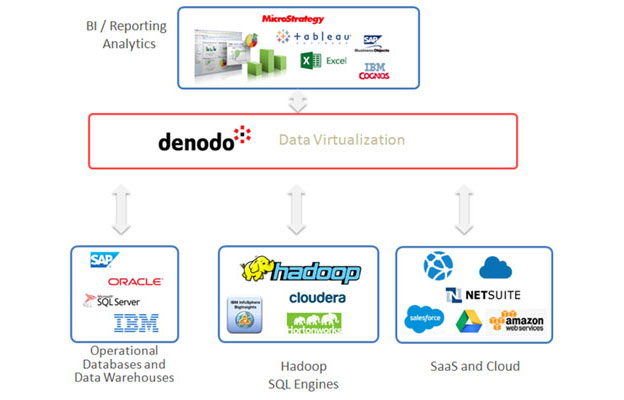
Figure 1: In the “Logical Data Warehouse” and “Logical Data Lake approaches, a Data Virtualization system provides unified reporting and governance over multiple data sources, which typically include one or several physical data warehouses or data marts, Hadoop-based systems, operational databases, SaaS applications (e.g. Salesforce), etc.
The appeal of the Logical Data Lake and Logical Data Warehouse comes from the huge time and cost savings obtained in comparison to the “physical” approach, where all data needs to be previously copied to a single system. Replicating data means more hardware costs, more software licenses, more ETL flows to build and maintain, more data inconsistencies and more data governance costs. It also means a much higher time to market. In turn, the logical approaches leverage your existing systems, minimizing or removing the need for further replication.
Nevertheless, in these “logical” approaches, the data virtualization server needs to execute distributed queries across several systems. Therefore, it is natural to ask how well those queries will perform compared to the “physical” case.
As we have shown in the aforementioned posts, even complex distributed queries that need to process billions of rows can be resolved by moving very little data through the network, provided we use the right optimization techniques. Now, it is time to quantify the performance of these techniques using a real example!
Consider the simplified Logical Data Warehouse scenario shown in Figure 2. As you can see, we have information distributed across three different systems: the Netezza system containing sales information (approx. 290 million rows), the Oracle database containing customer information (approx. 2 million rows), and the SQL Server database containing product information (approx. 200 thousand rows). The schemas and data of these tables are defined by TPC-DS, the most important standard industry benchmark for decision support systems.
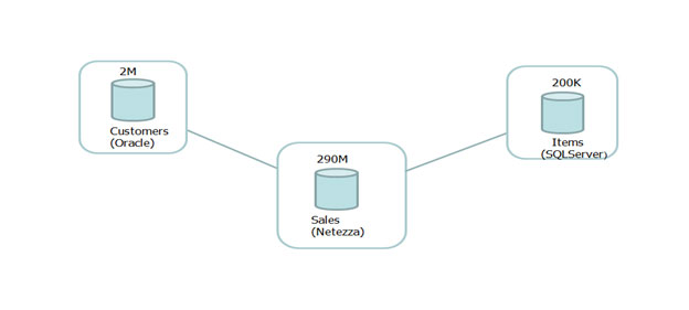
Figure 2: A simplified “Logical Data Warehouse” scenario. Sales, customer and products data is distributed across three different systems.
The following table shows the results obtained by executing some common decision support queries in both, the “logical” scenario (using Denodo 6.0 as a data virtualization tool on top of the data sources) and a “physical” scenario, where all the data from the other data sources has been previously replicated in Netezza.
| Query Description | Rows Returned | AVG Time Physical (all data in Netezza) | AVG Time Logical (data distributed in three data sources) | Optimization Technique (automatically chosen by Denodo 6.0) |
| Total sales by customer, including customer data | 1,99 millions | 20975 ms | 21457 ms | Full group by pushdown |
| Total sales by customer and year between 2000 and 2004, including customer data | 5,51 millions | 52313 ms | 59060 ms | Full group by pushdown |
| Total sales by item and brand, including items data | 31,35 thousands | 4697 ms | 5330 ms | Partial group by pushdown |
| Total sales by item where sale price less than current list price, including items data | 17,05 thousands | 3509 ms | 5229 ms | On the fly data movement |
As demonstrated in column 1, the queries do not use highly selective conditions. Actually, rows 1 and 3 do not specify any filtering condition at all, so they need to process hundreds of millions of rows in the respective data sources. In the second column, you can see that the queries return millions of rows as final result. A comparison of column 3 and 4 shows actually how small the performance difference is between the two approaches.
Finally, the last column of the table specifies the optimization technique (described in my previous posts) automatically chosen by Denodo to execute each query.
Conclusion
In this series of posts, we have compared the performance of the Logical Data Warehouse and Logical Data Lake approaches to the “physical” approaches, where all data is previously replicated in a single system. We have shown that the logical approach can obtain performance comparable to the physical approach, even in large BI queries, processing billions of rows which do not use any filtering conditions. The key to achieve this is a data virtualization system capable of intelligently deciding and applying a set of optimization techniques that minimize data transfer through the network. In addition, the logical approaches avoid the large amount of time and effort often associated with replication-based approaches, provide much shorter times to market, and constitute a single entry point for unified security and governance. We think this insight is of capital importance for current and future BI and Big Data architectures.

- Performance in Logical Architectures and Data Virtualization with the Denodo Platform and Presto MPP - September 28, 2023
- Beware of “Straw Man” Stories: Clearing up Misconceptions about Data Virtualization - November 11, 2021
- Why Data Mesh Needs Data Virtualization - August 19, 2021
These data sources typically include one or several physical data warehouses, a Hadoop Cluster, SaaS applications and additional databases. Where did you get this information?
Hi grenefex,
Those are the typical data source types we find in the “Logical Data Warehouse / Data Lake” deployments of our customers.
Best regards,