
The amount of data a company can manage these days is huge, but making use of these data for analytics and decision-making can be hard and expensive using traditional approaches.Traditional architectures like data warehouses and data lakes rely on storing all data in a centralized repository. This means long and rigid ETL processes and high costs in hardware infrastructure, security and maintenance. Besides, sometimes the replication is not even possible due to security policies or simply because the data source is too big.
On the other hand, a logical architecture like data virtualization allows accessing all data in real time from a single point minimizing replication. The virtualization layer shows the appearance of a regular relational database but it has the ability to access and extract data from almost all sort of data sources (data warehouses, relational databases, Hadoop clusters, web services, …) and publish the results in multiple formats like JDBC, ODBC or REST data services.
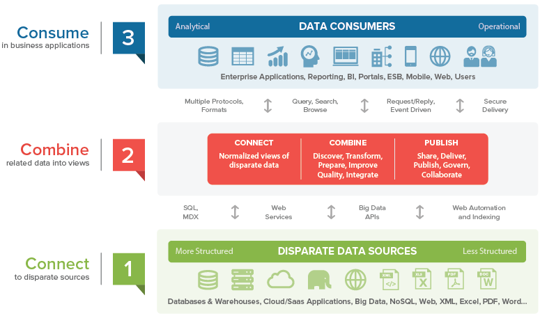
With this approach data can remain in its original sources, and when the virtualization layer receives a query, it identifies the operations corresponding to each source, sends the necessary subqueries to these disperse and heterogeneous sources, retrieves and combines the data and returns the final result. This offers a single point of access and security to maintain, and an abstraction layer that disconnects the actual hardware architecture storing the data from the business applications. This not only reduces costs but also provides big time savings on the development of new projects.
As you can imagine, one of the biggest challenges for a virtualization system like this is achieving a good performance even when it has to transfer data from several sources. Because of this, it is crucial to have a powerful query optimizer capable of choosing the best execution strategy for each query.
The query optimizer works in a way that is transparent to the user and is in charge of analyzing the initial query and exploring, comparing and deciding among the different equivalent execution plans that could obtain the desired result.
It automatically evaluates different possible execution plans estimating the costs associated with each one in terms of time and memory consumption to decide which one is better for that specific query. In order to achieve accurate estimations it must take into account not only the estimated rows that it would need to transfer from each source but also information like if the data source will use an index or if the data source will process a certain operation in parallel.
Let me show you a few examples to fully understand the impact that the optimizer decisions can have in the performance. I will use a similar use case from previous posts, but this time I will include some additional execution plans to consider. Most of them are already included in Denodo Platform version 6.0 but I will also describe a new strategy included in Denodo Platform version 7.0.
The use case consist of a retailer company that stores the information about its 2 million customers in a CRM, and the information about the sales in two different systems:
- An enterprise data warehouse (EDW) containing sales from the current year (290 million rows) and,
- a Hadoop system containing sales data from previous years (3 billion rows).
Let’s say that we want to obtain the total sales by customer name in the last two years.
The first figure shows the mechanism a simple data federation engine would use to resolve this query.
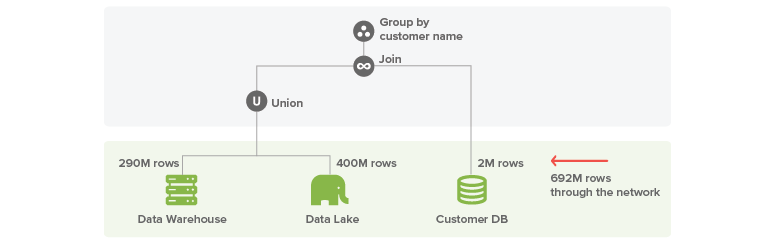
It retrieves the 290M rows from the data warehouse and 400M rows (corresponding to the previous year) from the Hadoop system. Then it joins these data with 2M customers coming from the CRM. This means transferring 692M rows through the network and then performing the joins and aggregation at the virtualization system: it is easy to see this will take minutes.
A more sophisticated data virtualization engine can optimize this plan by sending a partial aggregation to each sales source. This is, instead of retrieving all the sales from the last two years, it can ask for the total sales by customer from the last two years. Both systems will perform this partial aggregation very efficiently and this partial group by will return in the worst case one row for each customer, 2M rows from each source. Then, it can join the data and aggregate the partial results by customer name to get the final result.
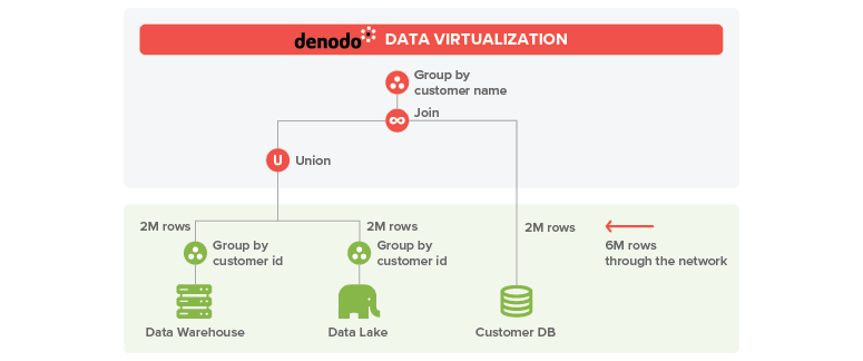
With this improvement, you just need to transfer 6M rows through the network, and the execution times will be reduced in orders of magnitude. This technique is usually called aggregation pushdown.
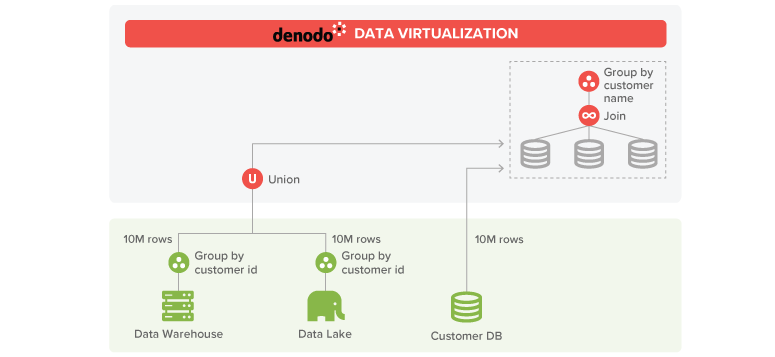
Now imagine that instead of the total sales by customer, we want the total sales by customer country during the same period, and we have customers in 10 different countries. Following a similar strategy, we can push a partial group by operation to each sales data source aggregating by customer_id, then join the partial sales aggregation with each customer and perform the final aggregation by country. This option would also transfer 6M, one from each source.
However, we could also think on another possible execution plan:
We can create a temporary table in both Hadoop and the data warehouse systems with the data from customer. Then, we can push both the join and the group by under the union and let each source perform the join and group by operations.
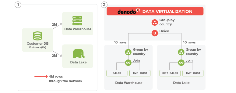
This way, each source would send 10 rows (one by customer country) from its partial aggregation, and the data virtualization layer would just need to aggregate this partial results to get the final result.
This option has the extra cost of creating a temporary table and inserting 2M rows in the two sources (in parallel) but the advantage that both the data warehouse and the Hadoop cluster can resolve joins and aggregations very efficiently and then they will transfer just 20 rows back to the DV server.
Let’s turn the scenario a bit harder. Now imagine that we want to obtain the total sales by customer, but instead of 2M customers we have 10M customers. In this case this second strategy may not be the best one, as we would need to read 10M customers, insert the 10M rows in each source, transfer 20M coming from the partial aggregations and then perform an aggregation with 20M rows.
The first strategy, aggregation push down, could be a good option, but we would need to transfer 30M rows in total (10M from customer and 10M from each partial aggregation) and then perform a group by with 20M rows.
Although this is much better than the naive approach, aggregating 20M rows can be a high-memory consuming operation, so we would need to swap these data to disk to avoid monopolizing the system resources.
Denodo Platform version 7.0 can greatly optimize this type of operations by using massive parallel processing (MPP). To achieve this, Denodo leverages the modern in-memory features of SQL-on Hadoop systems like Spark, Impala or Presto. Let’s say we have any of these systems running on a cluster connected to Denodo through a high-speed network. When the optimizer detects that Denodo will need to perform costly operations on large amounts of data, it can decide to stream the data directly to the cluster to perform them using massive parallel processing. In our example, Denodo can transfer the data from customer (10M) and the partial sales aggregations results (10M each) to this cluster and resolve there the join and group by operations to obtain the final result. With this option, the join and group by operations will be much faster as each node of the cluster will work in parallel over a subset of the data.
These are just some of the possible strategies that the Denodo optimizer can apply to resolve a query. You can infer from the previous examples that it does not exist a magic strategy which is optimal for all cases. Therefore, a powerful query optimizer must be capable of: reordering operations to minimize the data transfer; considering the right execution alternatives; and making accurate estimations, taking into account the particularities of the data sources.
Using these techniques a data virtualization system can achieve very good performance even when it has to deal with large and distributed data sets. You can find real execution times using Denodo Platform version 6.0 in this previous post and, in the following posts we will provide new numbers for the upcoming version 7.0.
In conclusion, when considering a data virtualization solution for logical analytics architectures, keep in mind that the query optimizer plays a crucial role in the performance and the power of this optimizer can truly make a difference among competitors.

Among her contributions to the Denodo Platform she has led the design and development of some of the key features of the query optimizer module.
- Using AI to Further Accelerate Denodo Platform Performance - September 9, 2021
- Increase the Performance of Your Logical Data Fabric with Smart Query Acceleration - October 28, 2020
- Achieving Lightning-Fast Performance in your Logical Data Warehouse - November 6, 2017